SINDY

This work is a re-creation of a symbolic regression method from Brunton and Kutz. The article is meant to be a quick summary of this method.

All figures, equations, examples and code are a work of my own. Only the idea has been borrowed from the paper.

Introduction

Data driven methods are the modern day equivalent to Poincare’s work in the 19th century. A characteristic feature of these methods is determining the equations of motion underlying a given dynamical system, exclusively from time dependent observables, measured from that system.

Consider this generic form of a dynamical system.

\[\begin{align} \frac{dx(t)}{dt} = f(x(t)) \\ x(0) = x_0 \in \mathbb{R}^d \end{align}\]

Given \(X := [x(t_1),x(t_2),...,x(t_N)]\), we would like to infer \(f\) either symbolically or numerically.

SINDY is a symbolic regression algorithm that identifies \(f\), provided one has access to the most apposite bases set, say \(\mathcal{B}\), that spans the function space \(\mathcal{F} \ni f\). It’s usually the case that for most systems, knowledge of \(\mathcal{B}\) is sparse at best; raising serious questions about the practicality of this method for data arising from real world applications. Nonetheless it is a nice method where one has expert knowledge about the system. The algorithm has four main steps.

Algorithm

Evaluate \(\dot{X} := [\frac{dx(t_1)}{dt},\frac{dx(t_2)}{dt},...,\frac{dx(t_N)}{dt}] \in \mathbb{R}^{d \times N}\) using a sufficiently robust finite difference scheme.
Choose a bases set \(\mathcal{B} := \{b_1(x), b_2(x), ..., b_k(x)\}\) of functions.
Evalute \(\Theta(X) := \begin{bmatrix} b_1(x(t_1)) && ... && b_1(x(t_N)) \\ \vdots && && \vdots \\ b_k(x(t_1)) && ... && b_k(x(t_1)) \\ \end{bmatrix} \in \mathbb{R}^{k \times d \times N}\)
If \(\dot{X} = K \: \Theta(X)\) where \(K \in \mathbb{R}^{k}\). Solve for \(K\) using linear least squares and a sparsity inducing regularizer.

Examples

Here the algorithm is applied to commonly recurring examples in literature – Lorenz 69 attractor and a Lotka-Volterra model.

Lorenz 69 attractor

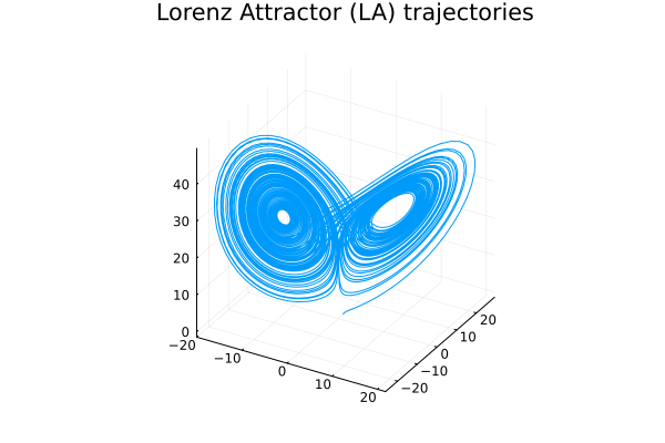
The following non-linear ODE with a specific configuration of parameters has been the poster-child of chaotic attractors for several decades now.

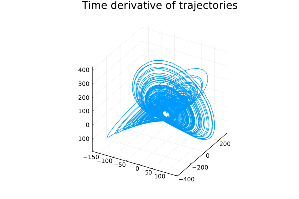
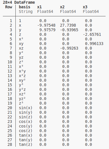
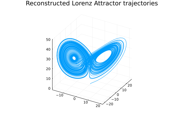
\[\begin{align} \dot{x}(t) = \sigma (y - x)\\ \dot{y}(t) = x(\rho - z) - y\\ \dot{z}(t) = xy - \beta z\\ \sigma = 10 \\ \rho = 28 \\ \beta = \frac{8}{3} \\ \begin{bmatrix} x_0 \\ y_0 \\ z_0 \end{bmatrix} = \begin{bmatrix} 1 \\ 0 \\ 0 \end{bmatrix} \\ t \in [0,100] \end{align}\]

Viewed clockwise, the figure below shows i) Trajectories of the attractor obtained from a numerical integrator, ii) Time derivative of the trajectories, iii) Chosen bases functions \(\mathcal{B}\) and the corresponding weights and iv) the reconstructed attractor.

Lotka Volterra model

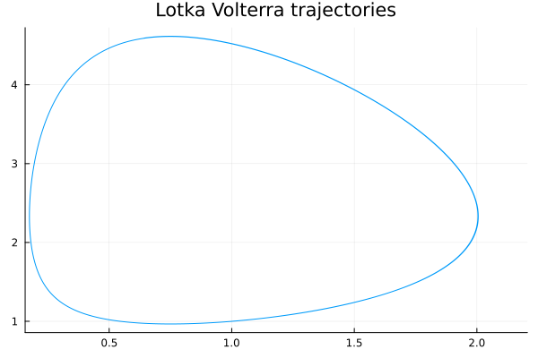
Prey predator models are the staple for several ecological, biological and even plasma physical applications. A common model with a single species of prey and predator is shown below.

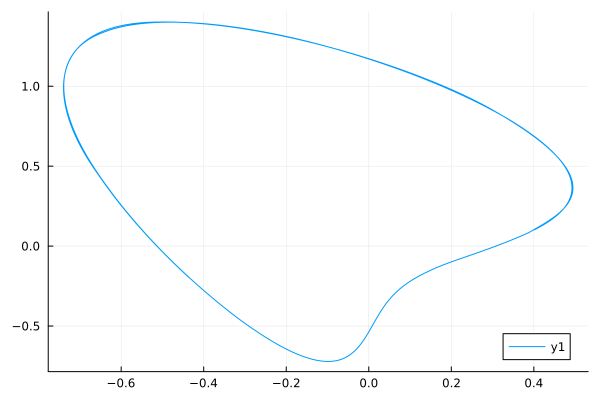
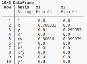
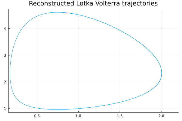
\[\begin{align} \dot{x}(t) = \alpha x(t) + \beta x(t)y(t) \\ \dot{y}(t) = \gamma x(t)y(t) - \delta y(t) \\ \alpha = 0.7 \\ \beta = -0.3 \\ \gamma = -0.3 \\ \delta = 0.4 \\ \begin{bmatrix} x_0 \\ y_0 \end{bmatrix} = \begin{bmatrix} 1 \\ 1 \end{bmatrix} \\ t \in [0,100] \end{align}\]

Akin to the Lorenz attractor, the SINDY algorithm is used to infer the bases weights and the trajetories are then reconstructed.

Code

These results can be reproduced with the following code. (Documentation coming soon.)