Multi-output Gaussian processes
Introduction
Gaussian processes are a popular Bayesian learning framework.
A typical learning problem consists of approximating an approximation \(\hat{f}\) to the function \(f:x \mapsto y \quad \forall x,y \in \Omega \subset \mathbb{R}^d\), given evaluations of the function at certain input points, that is \(\mathcal{D} = \{(x_i, f_i) : i \in \mathbb{N}\}\).
Bayesian inference assumes that the input \(x\) and the outputs \(y\) are random variables. These densities are related by
\[P(x,y) = P(y | x) P(x) = P(x | y) P(y)\]Note that we do not have a closed form for any of these probability functions and estimating probability densities from data is in itself a hard problem. Instead, we make guesses about what these functions might be. Historically, each of these probability functions have their own names, namely
- \(P(y)\) – Prior
- \(P(x | y)\) – Likelihood
- \(P(x)\) – Marginal
- \(P(y | x)\) – Posterior
Commonly, one assumes a functional form for the prior. The posterior is the updated version of the prior, once we have seen the reference data.
Gaussian processes
If the likelihood and prior are Gaussian, then the Bayesian inference framework is a Gaussian process framework. In this case, the posterior has a closed form. I will discuss this in this section and write down the general inference procedure using Gaussian processes.
Let \(y:=f(x) \sim GP(\mu(x), \kappa(x,x';\theta))\) and let the discrete observations of \(x,y\) be stacked into tall vectors \(X,Y\) respectively. If one is interested in evaluating \(f\) at a new point \(x\), one need only compute the expectation of \(\mathcal{N}(\hat{\mu}_k, \hat{\Sigma}_k)\) such that
\[\begin{align} \hat{\mu} = K_{xX} \: (K_{XX} + \Lambda)^{-1} Y \\ \hat{\Sigma} = K_{xx'} - K_xX \: (K_{XX} + \Lambda)^{-1} K_{Xx'} \end{align}\]Here \(K_{ab}^{ij} = \kappa(a[i],b[j];\theta_{k-1})\).
Algorithm
Given:
- Covariance kernel \(\kappa\).
- Reference data \(X,Y\)
- Query points \(x\)
- Threshold \(\epsilon\)
- Noise covariance \(\Lambda\)
For a given \(k\):
- Evaluate \(K_{XX}\)
- Compute \(y_k := K_{XX} \: (K_{XX} + \Lambda)^{-1} Y\)
- Obtain discrepancy \(\mathcal{E}_k := \| y_k - Y\|\)
- Compute \(G_k := \nabla_{\theta_{k-1}} \mathcal{E}\)
- Update \(\theta_{k} := \theta_{k-1} - \alpha * G_k\)
Until discrepancy \(\mathcal{E} < \epsilon\):
- Do the previous 6 steps.
- Increment \(k\)
Then,
- Compute mean \(\hat{\mu}\) and covariance matrix \(\hat{\Sigma}\) with optimized \(\theta\).
- Return \(\mathcal{N}(\hat{\mu},\hat{\Sigma})\)
This procedure approximates any given function \(f\) from its samples. To illustrate this, consider the following example.
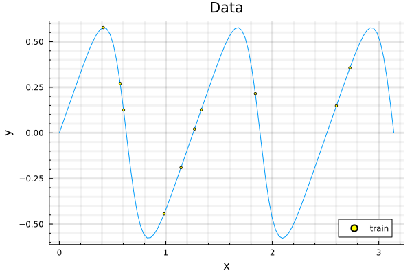
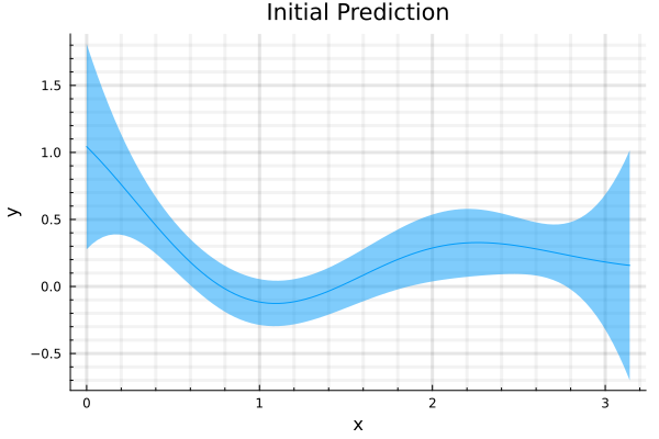
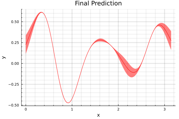
With a squared exponential kernel, the sinusoidal function, before hyperparamter optimization is shown in the second figure and the prediction after optimization, is shown in the third. Note that variance in the prediction is high, for out of sample distributions as it should be.
Multi-output Gaussian processes
The algorithm from the previous section is readily transferable to vector valued functions as well; with the added change that one uses kernel functions that are better suited for this application. A comprehensive review of vector values GP kernels can be found in Alvarez.
In the rest of the section, I will approximate the trajectories of the Lorenz attractor
\(\begin{align} \frac{d}{dt}\begin{bmatrix} x \\ y \\ z \end{bmatrix} = \begin{bmatrix}\sigma (y - x)\\ (\rho - z) - y\\ xy - \beta z \end{bmatrix} \\ \sigma = 10, \: \rho = 28, \: \beta = \frac{8}{3} \\ \end{align}\) with suitable initial conditions. One such trajectory we are interested in, looks like

Independent GPs – IGP
Three independent GPs, each approximating \(x(t), y(t), z(t)\) require 100 randomly sampled points to make predictions (shown below) with a Matern kernel.

This would be the minimum possible predictive accuracy that vector valued GP models need to realize. The divergence in \(\epsilon\) for \(t>5.0\) is due to out of sampling error.