(Original Research) Latent space Bayesian Waveform Inversion

Introduction

Waveform inversion concerns reconstructing velocity fields from remotely measured wave signals. It has been common practice to optimize for velocity fields parameterized as indicator functions. Considering the ill-posed nature of inversion, the trend is to turn to Bayesian inversion methods, which can be formulated as well posed problems. In addition, Bayesian methods provides one, an estimate of the uncertainity in prediction, which is ever so crucial, should waveform inversion be used for resource sensitive applications.

Despite all evidences pointing towards adopting Bayesian parameter estimation for waveform inversion, it is still not common practice in the FWI community; largely because Bayesian methods are extremely expensive for models with large parameters.

In this work, we use the time honored practice of seeking latent space representations for families of velocity fields. Subsequently we demonstrate that Bayesian waveform inversion in these latent spaces becomes computational tractable.

Latent spaces

We begin with some observations. More specifically, we consider some velocity fields that are commonplace in the inversion literature – seismic and otherwise.

Fourier space representations

Initially, we seek Fourier space latent representation of the fields. Initial observations indicate that one can do away with more than 80% of the Fourier bases functions and still obtain a qualitatively good estimate of the velocity field at the cost of mapping to and back from the Fourier space. (This is realized with fft.)

Primitives

Velocity classes

One should note that, for discontinuous functions, high frequency Fourier bases functions become increasingly relevant. While, this was not so debilitating for the examples in the Primitive section, it is clear that seismic velocity fields cannot be robustly parameterized.

Learned latent space representations

This leads us to learning the latent space representations using variational autoencoders.

Autoencoders

But let’s initially review autoencoders. Autoencoders are approximation methods for learning a latent space representation \(z\) for a given vector \(x\) in the observable space. The latent space representation is sometimes called an embedding. A generic autoencoder consists of – an encoder and a decoder (as shown below).

Any \(x\) is hierarchically projected into a lower dimensional space upto the latent space using a dense fully connected neural network. This can also be realized using other network architectures such as CNNs and GNNs which can incorporate more inductive bias. The decoder is the mirror image of an encoder and aids in the reconstruction \(z \mapsto x\).

For instance, a reconstruction of the MNIST handwritten images, by sampling from the latent space and reconstructing it back, is shown below. Here \(x \in \mathbb{R}^{28 \times 28}\) and \(z \in \mathbb{R}^2\). Coincidentally, the MNIST digits can be viewed as spline shaped defects embedded in the domain of interest (similar to the primitives in the Fourier representations section.)

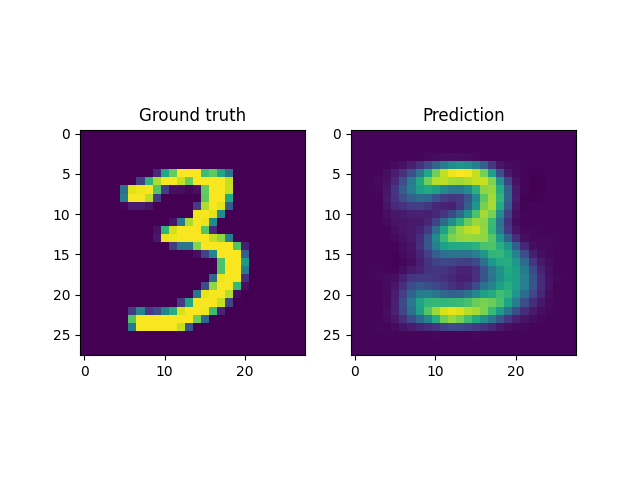
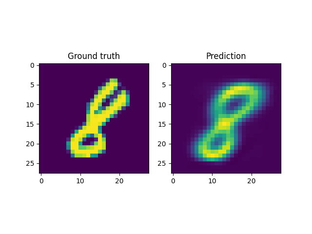
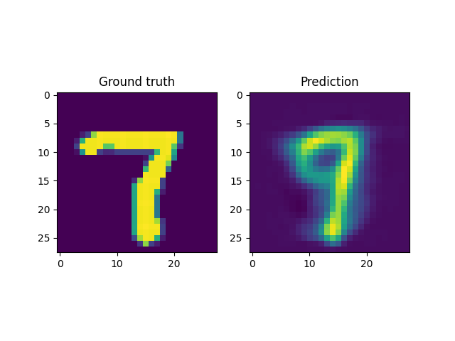
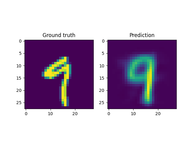
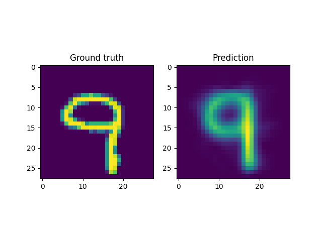
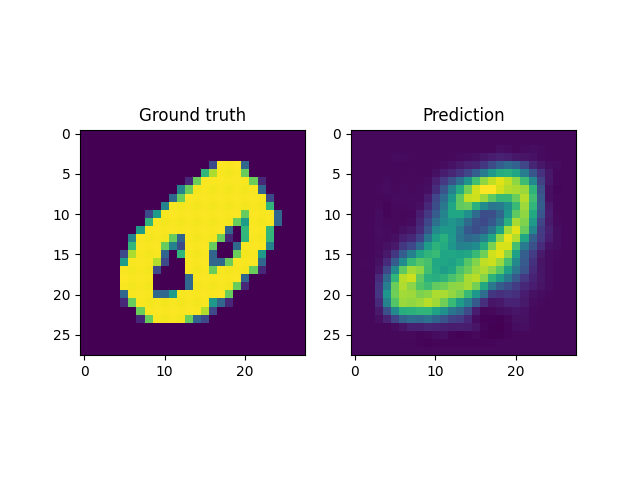
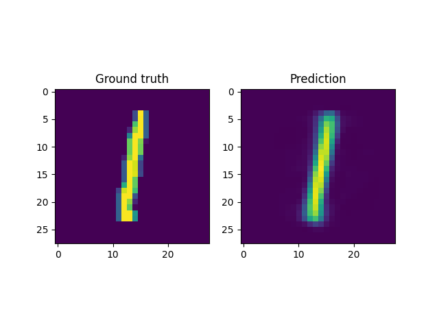
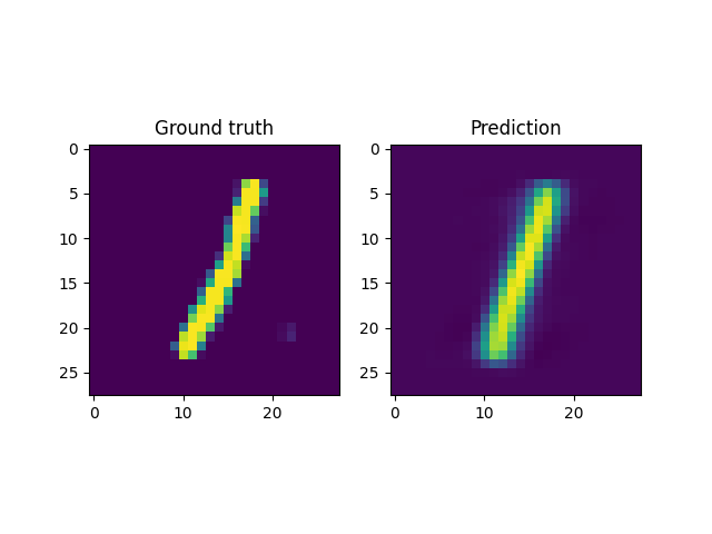
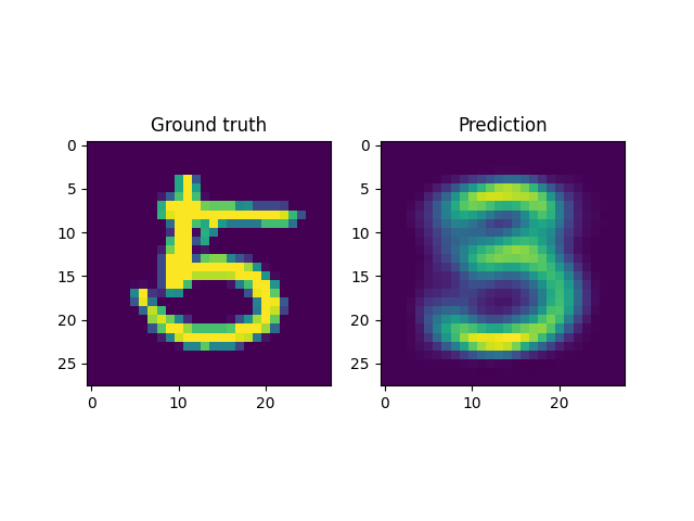
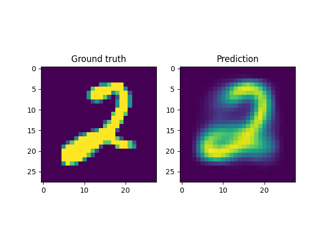
However, autoencoders are also notoriously hard to train; with gradient based optimization algorithms trapping themselves often in local minima.

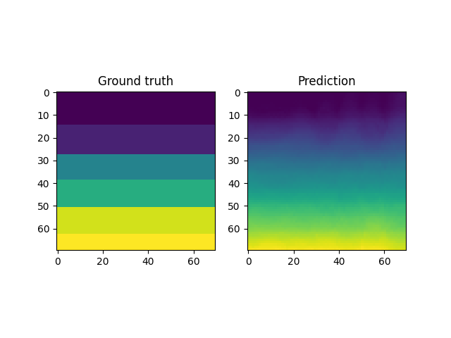
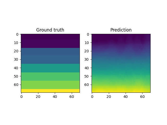
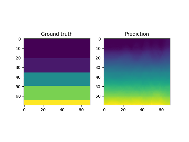
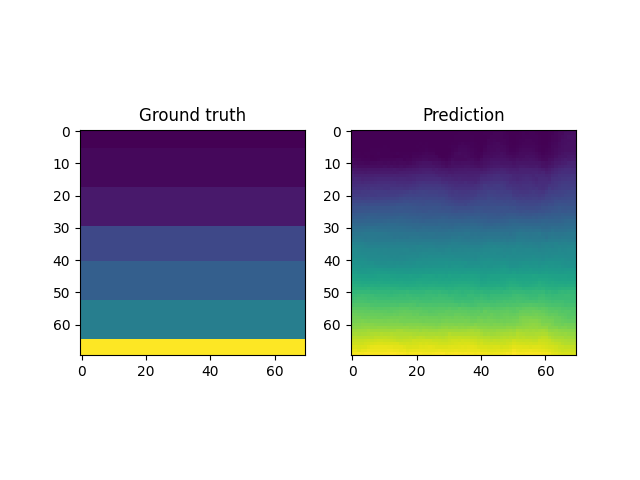
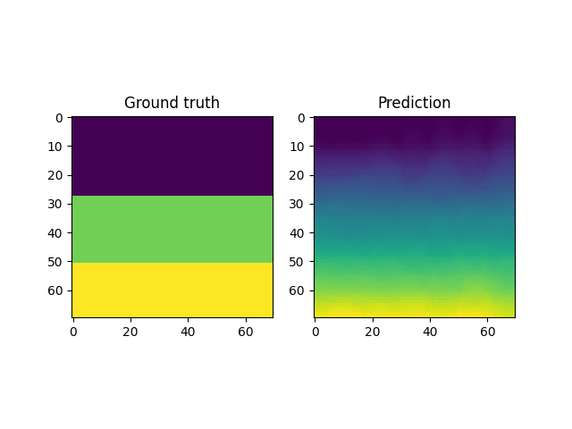
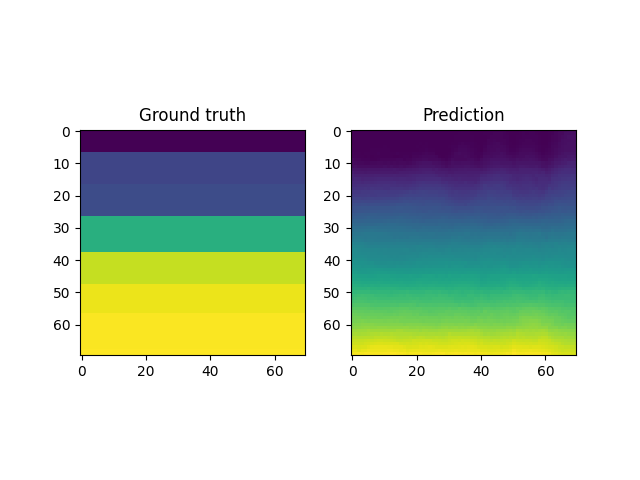
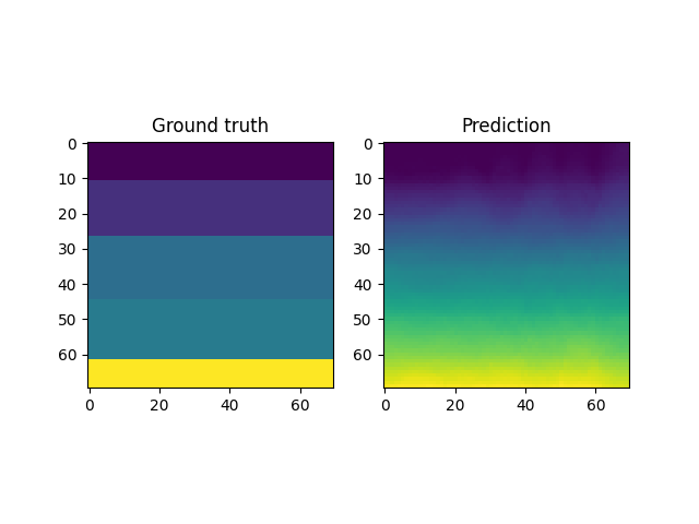
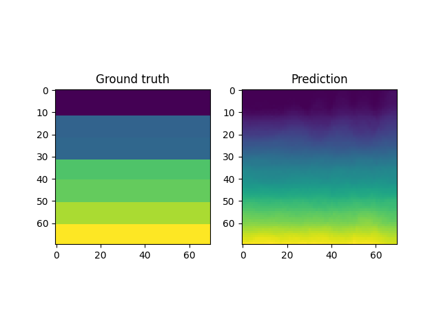
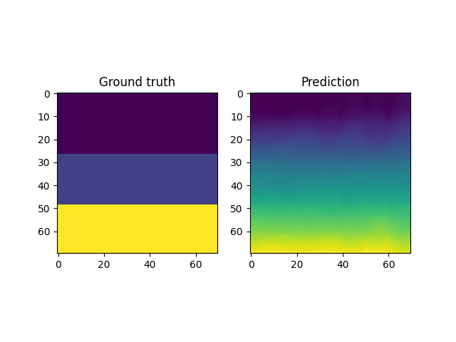
This is the case with the results above, where the embeddings cannot sufficiently represent the different velocity fields faithfully. In light of this, it makes more sense to look into VAEs which have been shown to be more robust to this issue.

Variational Autoencoders

Variational Autoencoders (VAEs) approach this representation learning problem from a Bayesian perspective. It assumes that there exists a joint probability distribution \(p(x,z)\). Then for a prior over \(z, p(z) \sim \mathcal{N}(\mu, \Sigma)\), one can find predictors for \(x\) using Bayes rule. That is,

The marginal \(p(x)\) is untractable for most practical scenarios. However, one can use variational inference to estimate the posterior \(p(z|x)\) with \(q_{\theta}(z|x)\). That is, one can optimize for the parameters \(\theta\) by minimizing the Kullback-Leiber (KL) divergence between the two distributions. The backward KL divergence in this case is given by

This ofcourse is intractable, since it still contains the marginal \(p(x)\). Fortunately the above expression can be re-written as follows

Minimizing the left equation on the left hand side, also minimzes the KL divergence, since

This is the evidence upper bound or the EUBO, which is actually tractable. In the context of the autoencoder,

1. \(q(z|x)\) is the probability distribution over predictions from the encoder.
2. \(p(x|z)\) is the same for the decoder.
3. \(p(z) \sim \mathcal{N}(\mu, \Sigma)\) is the prior.

The general architecture of a VAE is as follows. Here, the output of the encoder is the mean \(\mu\) and the covariance matrix \(\Sigma\) of a multi-variate normal distribution \(\mathcal{N}\). The samples from \(z \sim \mathcal{N}\) constitutes the latent space variable.

Training the VAE comprises minimizing the EUBO, for which one needs to make a few assumptions.