Parsimoniuously learning Koopman generators
Greens function based methods for inferring Koopman generators.
Deterministic Dynamical system
Consider a dynamical system, given by
\[\begin{align} \label{eq:DS} \frac{d}{dt} x(t) = f(x(t),t) \\ x(0) = x_0 \in \mathbb{R}^d \\ t \in \mathbb{R}^{+} \\ f: x \times t \mapsto \mathbb{R}^d \end{align}\]\(f\) in general is assumed to be an arbitrary non-linear function. The Koopman operator framework is based on this following insight:
Followingly, let \(\phi\) be an observable of the dynamical system, which is commonly chosen to be a real or complex valued function. That is
\[\begin{equation} \phi : x \mapsto \mathbb{R} \textrm{ or } \mathbb{C} \end{equation}\]With these considerations, the Koopman operator formulation of (\ref{eq:DS}) is
\[\begin{equation} x(t) := \Phi_t (x_0) = [\phi^{-1} \circ K^t \circ \phi](x_0) \end{equation}\]Here \(K^t\) is the family of Koopman operators corresponding to time \(t\).
Motivated by the temporal dependance of \(K\), it is normal to ask : Can one define a time dependent differential equation that generates the family \(K^t\)?
For any \(\tau, \eta \in \mathbb{R}^{+}\), consider the following:
\(\begin{align} \lim_{(\tau-\eta) \mapsto 0} \frac{1}{\tau - \eta} \left[K^{\tau} \circ \phi - K^{\eta} \circ \phi\right] \end{align}\) Or equivalently, \(\begin{align} \label{eq:generator} \frac{d}{dt}\phi(x(t)) = \left[\frac{d \phi}{dx}(x(t))\right]^T f(x(t),t) \end{align}\)
Right hand side of equation (\ref{eq:generator}) is the Koopman generator for a vector field \(f\). Analytical solutions to (\ref{eq:generator}) seldom exist, due to the non-linearity of \(f\).
Green’s function formulation
The generator is fortunately a linear operator.
\[\begin{equation} \mathcal{L} \: \Box := \sum_{i=1}^{d} f_i \frac{d}{dx_i} \Box \end{equation}\]Intuitively, it is known that for any linear operator \(\mathcal{L}\) there exists a Green’s function \(\mathcal{G}\).
In this case,
\[\begin{align} \frac{d}{dt}\phi(x(t)) = \mathcal{L} \phi(x(t)) \\ \end{align}\]with solution
\[\phi(x) = \int_{\Omega} \mathcal{G}(x,y) \: \frac{d\phi(y)}{dt} \: dy\]Existence of \(\mathcal{G}\) for \(\mathcal{L}\)
WIP
Learning \(\mathcal{G}\)
There are a number of alternatives here to effectively learn the Green’s function. Almost all these methods invariably involves using a neural network to parameterize \(\mathcal{G}\). Some of them include.
- Learning \(\mathcal{G}\) in the Fourier space.
- Learning \(\mathcal{G}\) in Euclidian space with deep neural networks.
WIP
- Learning \(\mathcal{G}\) in Euclidian space with sampling neural networks.
WIP
Examples
In the following, the efficacy of our method is compared with EDMD and gEDMD based on two metrics.
We demonstrate this on several examples that have appeared in literature surrounding Koopman operators.
1. Systems identification
Lorenz 69 attractor
Lotka volterra
Van der Pol oscillator
2. Non-intrusive model order reduction
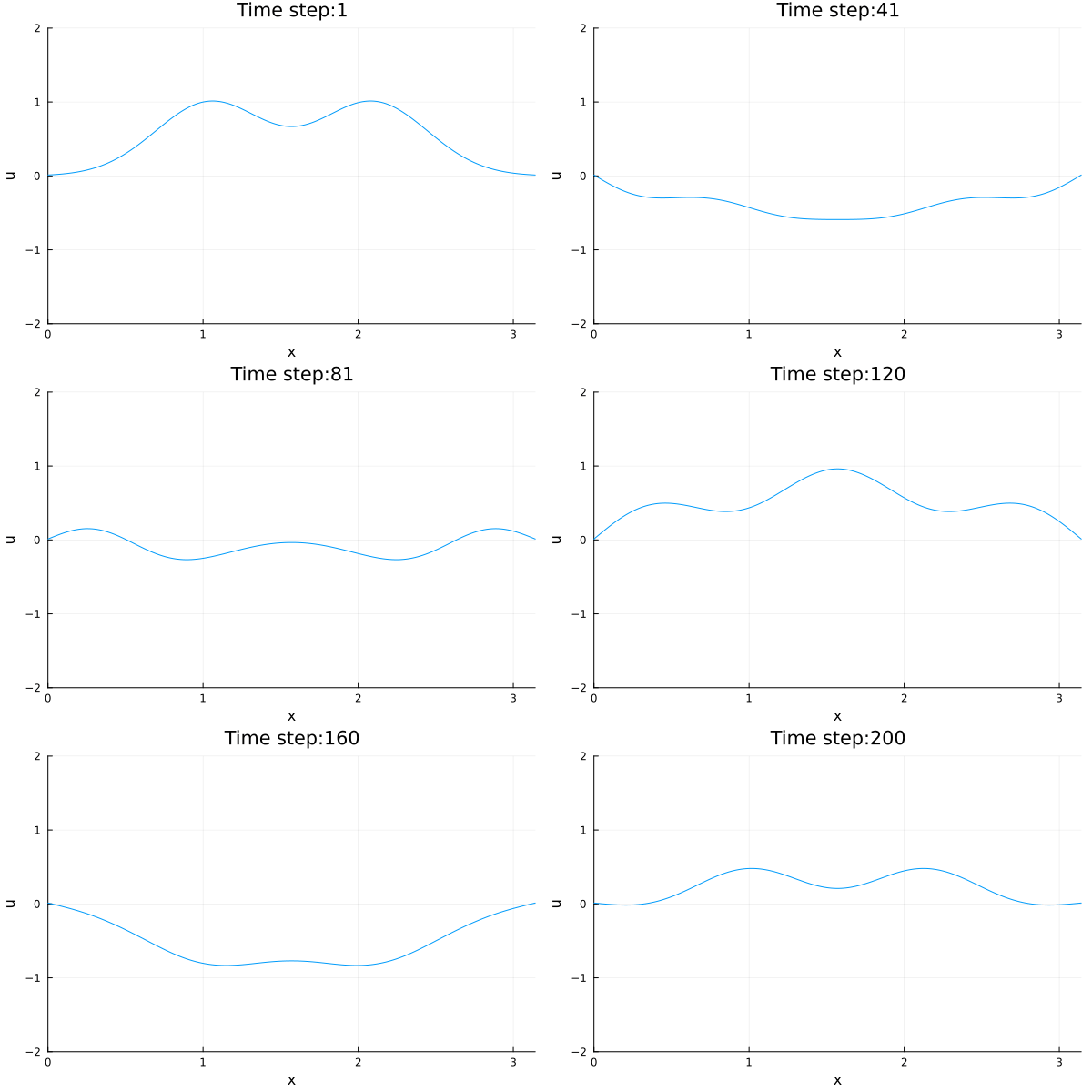
Acoustic Wave equation

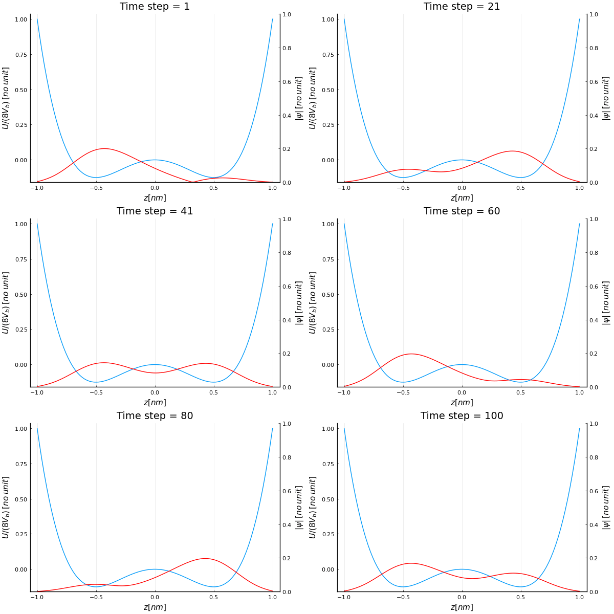
Schrodinger’s equation with double well potential
