FWI

Introduction

Full waveform inversion (FWI) is an effective technique to determine the subsurface mechanical properties of geological masses and engineering structures. It differs from other tomographic techniques in making use of the entire wavefield – the amplitude, phase and frequency, to estimate features with high resolution. Mathematically, it consists of minimizing the distance between a measured signal and an artifically simulated one.

Formally, let \(x \in \Omega\) be the domain of interest and let \(m_{o}(x)\) be an observable defined over \(\Omega\). Let \(A : m(x) \times x \mapsto u(x)\) be an operator, mapping the observable and the domain to the wavefield \(u\). (\(A\) is also known as the forward map.) If \(u_{o}(x)\) is the wavefield corresponding to \(m_{o}(x)\), then FWI is principally a minimization problem defined as:

\(\begin{equation} \label{eq:fwi} \arg \min_{m \in \mathcal{M}} ||u_{o}(x) - A(m(x),x)||_p \end{equation}\) where \(\mathcal{M}\) is the hypothesis space of candidate observables explored with respect to a suitable \(p\) norm.

Since its first formulation in 1977, much has been discovered about FWI with respect to the efficacy of optimizers (SGD vs quasi-Newton vs Newton vs Truncated Newton) and the choice of measures (\(L_p\) norm vs Wasserstein measure). Furthermore, advances in computing has also benefitted this discipline; with highly parallel solvers that operate on very large time and length scales.

Recently, machine learning based surrogates for forward maps are gaining traction due to their computational efficacy. Surrogates based on Neural Operators in particular have recently shown much promise for several applications in literature. In this work, we demostrate waveform inversion with such surrogates.

Problem Setup

Let \(\Omega \subset \mathbb{R}^{d \times d}\), where \(d\) is the grid resolution.

For a reference observable (velocity) \(m_0:\Omega \mapsto \mathbb{R}^{d \times d}\), let the waveform be \(u_0(x,t) = A(m_0(x),x) \:\: \forall x \in \Omega\).

Assuming that from an initial measurement (oracle), \(u_0(x_s,t) \:\: \forall x_s \subset \Omega\), is given, we are interested in numerically estimating \(m_0(x)\).

For instance, one could imagine the reference velocity \(m_0(x)\) as being :

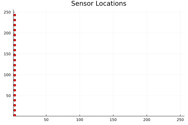
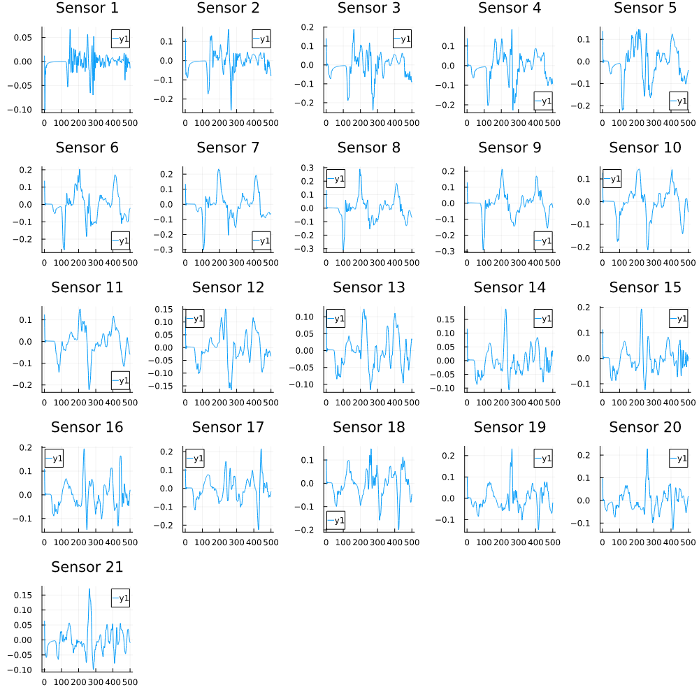
and the corresponding waveform sampled at seven different locations (sensors) in \(\Omega\) as

The optimization problem in \((\ref{eq:fwi})\) minimizes the distance betweem the above waveform (say) \(u_{m_0}\) and a waveform \(u\) obtained from a guessed observable \(m(x)\). Applications such as this, which repeatedly invoke an expensive computational routine such as the waveform map \(A\), are referred to as outerloop applications.

Depending upon the choice of basis used in discretization, computational routines involving \(A\) can be very expensive, usually due to the curse of dimensionality. Alternatively, we use Neural Operator surrogates for approximating \(A\).

Neural Operators

Let \(L u(x,t) = f(x,t)\) be an abstract partial differential equation for \(u \in \mathcal{U}\) and \(f \in \mathcal{F}\) (the output and input Banach spaces respectively). The operator \(L\) is said to be linear, if \(\forall f_1,f_2 \in \mathcal{F}\) and \(a,b \in \mathbb{R}\), \(L\:(a f_1 + b f_2) = a L f_1 + b L f_2\). It is known that for linear operators, there exists a propagator \(\mathcal{P}\) such that for any \(f \in \mathcal{F}\),

Neural Operators approximate \(\mathcal{P}\) by parameterizing it using a Neural Network. Hence, if one has a sufficiently many input-output pairs \(\mathcal{D} = (f_i,u_i)\), then learning the propagator \(\mathcal{P}\) is equivalent to learning the action of the operator \(L\) on all \(f \in \mathcal{F}\). We shall use this trick to approximate the waveform map \(A\).

Additionally, evaluating (\ref{eq:green}) is much more efficient on the Fourier space. To wit,

Approximating \(\mathcal{F}_x(\mathcal{P}(x,y,t,t'))\) using neural networks result in a computational framework that is known as Fourier Neural Operators in literature.

Approximation with Fourier Neural Operators

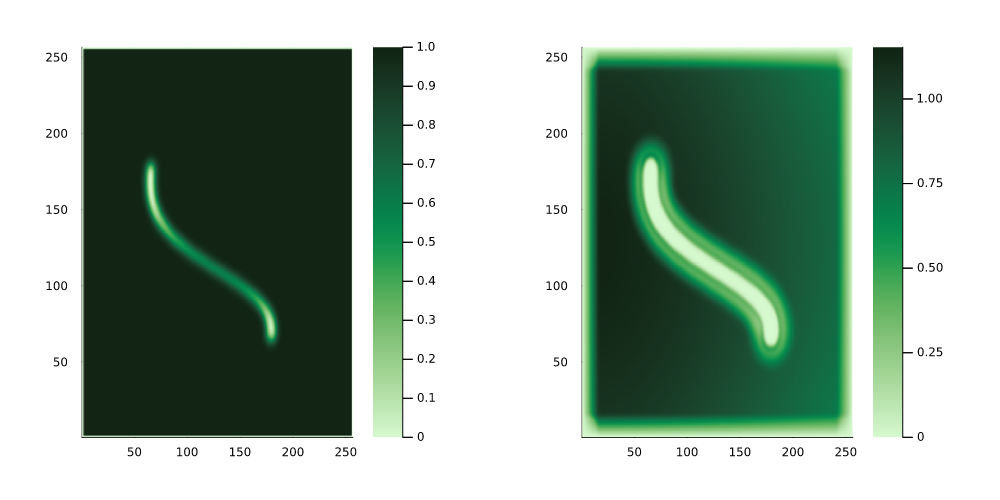
Fourier Neural Operators were trained on datasets generated from a full order finite difference approximation to the waveform map \(A\). Here, predictions from the surrogate for different velocity fields \(m(x)\) are presented.

The variety in \(m(x)\) is based on the primitive shapes such as splines, rectangles, circles and so forth. It is to be noted that, not all primitive shapes were used in training. Nevertheless, the FNO trained on a family of splines – sampled from a Gaussian process is capable of generalizing to sufficiently different function classes, as exemplified by its approximation over several seemingly disparate \(m\).

The evolution of the wavefield over a two dimensional domain, initially approximated by a finite difference approximation (simulation) and the FNO (surrogate) is juxtaposed for your perusal. Furthermore, the wavefield sampled at specific sensor locations (here the left end of the domain, as illustrated previously) is also presented.

Spline shaped velocity fields

Spline 1 [Not included in training].

Spline 2 [Not included in training].

Circular velocity fields

[Not included in training].

Rectangular velocity fields

[Not included in training].

Square velocity fields

[Not included in training].

Diagonal velocity fields

[Not included in training].]

Inversion

The results in the previous section indicate that the surrogates albeit with some bias, can qualitatively reproduce the action of a linear waveform map \(A\). One issue that is immediately obvious from the visualizations is the wavy nature of the predictions from the FNO. This is to be expected. As truncating the higher modes from the Fourier series of a function, is known to suffer from this problem. Alternatively, a Chebyshev expansion of the function can be used, but this remains outside the scope of this work.

Subsequently, we use this surrogate to invert artifically generated measurements (from the simulation), say \(\tau_{m_{ref}}\), inturn resulting in velocity field \(m_{ref}(x)\). In order to ensure, the waviness of the prediction from the surrogate, does not further ill-condition the problem, the prediction is smoothed using radial bases functions.

Parameterization

Prior to pursuing this, I will make a brief remark on how \(m(x)\) is to be parameterized.

Parameterization is a necessary here, as a dense mapping \(m:\Omega \mapsto \mathbb{R}\) suffers from the curse of dimensionality during gradient computation. Instead, radial bases sets are used to generate a one dimensional candidate function which is in-turn plotted inside \(\Omega\) yielding \(m_{can}\). The similarity measure between \(\tau_{m_{ref}}\) and \(\tau_{m_{can}}\) is now optimized with respect to the coefficients of these radial bases functions, say \(k\).

Let \(n\) be the number of radial bases functions. Then \(k \in \mathbb{R}^n\). Here, the velocity field is defined as follows: