MLP
Learning interaction potentials of many body systems.
Introduction
Machine learning potentials are surrogates for expensive electronic structure calculations. The use of these surrogates is justified on account of the iterative nature of MD simulations for several practical applications from drug design to material discovery. Training such machine learning models over molecular properties calculated for billions of atomic configurations, has been shown to provide sufficient generalization accuracy. In this work, I introduce a new way of training second and third generation machine learning potentials with a recently proposed sampling algorithm.
Workflow
A typical workflow for training machine learning potentials is illustrated below.

As an example, a molecule of sucrose is considered. Sucrose – \(C_{12} H_{22} O_{11}\) is a hydrocarbon ubiquitous in fruits, sugars and other sweetening agents. The goal of this workflow is to efficiently predict the molecular properties of sucrose for different positions of the carbon, hydrogen and oxygen atoms respectively.
Typically, several positions of atoms \(\textbf{R}\) and their atomic numbers \(\textbf{A}\) are concatenated into a single vector called an atomic descriptor – \([\textbf{R},\textbf{A}]\). It has been observed that encoding additional inductive bias, based on the physics of the system can improve the accuracy of the training procedure. Promptly, the atomic descriptors are mapped into a higher level descriptor coordinate \(\textbf{D}\). One should bear in mind, that the computational complexity of this descriptor map should be as low as possible. Finally, the descriptor coordinates \(\textbf{D}\) are mapped onto the space of molecular properties using a neural network.
Training this model, entails altering the parameters of the neural network iteratively until the predictions from the network and the reference data from electronic structure calculations match to an acceptable degree of accuracy.
Classification of machine learning potentials and molecular descriptors.
In 2021, Behler classified machine learning potentials, based on the choice the neural network architecture.
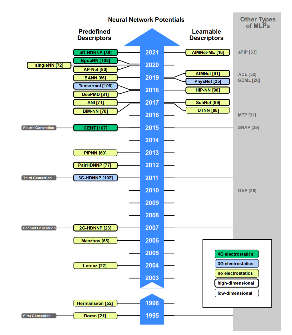
Furthermore, research into descriptors for machine learning potentials is also quite involved as illustrated in this phylogenic tree of molecular descriptors. (Adopted from this paper)
Contrbutions
In the light of this ubuquity, I choose two models, PairHDNNP from the third generation and DeepPMD from the fourth generation of neural network potentials. It should be stated, that these models do not represent the state of the art in “Surrogates for force computational in quantum chemistry”. Nonetheless, they are sufficiently recent to demonstrate the efficacy of our training algorithm. These models are trained on the MD17 dataset.
MD17 dataset
The MD17 dataset was first introduced along with the GDML model for inferring atomic forces. It consists of eight organic molecules with upto 21 atoms and 4 different chemical species, including
- Benzene
- Uracil
- Naphthalene
- Aspirin
- Salicylic acid
- Ethanol
- Toluene
For each of these molecules, several thousand atomic configurations \(R = \{R_i : i \in [1,m]\}\) along with the corresponding ground state energies \(E\) and the atomic forces \(F\), computed from density functional computations are furnished. This constitutes the core of the dataset.
..Insert figures of these molecules..
Inference models
Both the PairHDNNP model and DeePMD model have the following neural network architecture.

The atomic coordinates \(R_i\) are mapped to a local environment feature vector \(D_i\). This transformation is different for the two models. Individual deep fully connected neural networks \(N_i\) are used to approximate the local atomic energy \(E_i\). The total energy, \(E\), which is an extensive property is the sum of the individual atomic energies.
DeePMD models
Version 1
There are several iterations of the DeePMD model. In the first ever model , the local atomic environments, \(D_i\) are defined by the following map.
\[\begin{equation} \label{eq:DeepMD} D_i(...,R_i,...) = \begin{bmatrix} \dots &\dots &\dots& \dots \\ \vdots &\vdots &\vdots& \vdots \\ \frac{1}{r_{ij}} & \frac{R_{ij}^x}{r_{ij}^2} & \frac{R_{ij}^y}{r_{ij}^2} & \frac{R_{ij}^z}{r_{ij}^2} \\ \vdots &\vdots &\vdots& \vdots \\ \dots &\dots &\dots& \dots \\ \end{bmatrix}^{T} \in \mathbb{R}^{4 \times n} \end{equation}\]Here, information about the system, is sufficiently captured using all relative distances and displacements between the atoms.
Version 2
Subsequently, a more physically inspired descriptor with a cutoff parameter was proposed.
\[\begin{equation} \label{eq:DeepMD2} D_i(...,R_i,...) = \begin{bmatrix} \dots &\dots &\dots& \dots \\ \vdots &\vdots &\vdots& \vdots \\ \mathcal{s}(r_{ij}) & \frac{\mathcal{s}(r_{ij}) R_{ij}^x}{r_{ij}} & \frac{\mathcal{s}(r_{ij}) R_{ij}^y}{r_{ij}} & \frac{\mathcal{s}(r_{ij}) R_{ij}^z}{r_{ij}} \\ \vdots &\vdots &\vdots& \vdots \\ \dots &\dots &\dots& \dots \\ \end{bmatrix}^{T} \in \mathbb{R}^{4 \times n} \end{equation}\] \[\begin{equation} \label{eq:source} s(r) = \begin{cases} \frac{1}{r},& \text{for } r < r_{cs} \\ \frac{1}{r}\left(\frac{1}{2} cos\left[ \pi \frac{r-r_{cs}}{r_c - r_{cs}}\right] + \frac{1}{2}\right),& \text{for } r_{cs} \leq r < r_c \\ 0, & \text{for } r \geq r_c \end{cases} \end{equation}\]It should be noted that, both versions of the DeepMD descriptors are invariant with respect to translation and rotation. However, when two identical atoms in a molecule are permuted, the descriptor functions do vary.
HDNNP models
This drawback is overcome in the HDNNP descriptors. Here permutation invariance is built into the descriptor function by summing up over all possible configurations. This comes in two flavours – a two body descriptor and a three body descriptor. Higher body descriptors are possible, however this would render them computationally intractable.
Two body descriptors
Contrary to the previous descriptor, the local environment in this case is specified by a scalar.
\[\begin{equation} \label{eq:behler-2} D_i(...,R_i,...) = \sum_j e^{-\left(\frac{R_{ij} - R_c}{\sigma}\right)^2} s(R_{ij}) \end{equation}\]Three body descriptors
Model order Reduction methods
Borrowing ideas from reduced basis modeling, one can seek a low rank approximation for the potential energy. Such functions in the low dimensional space can be good descriptors, as it was recently demonstrated in the case of certain metallic elements.